Author: Raia Hadsell et al.
Paper Link: http://yann.lecun.com/exdb/publis/pdf/hadsell-chopra-lecun-06.pdf
Concept
The Beginning of Contrastive Loss
Notation
- Pairs of samples $\vec X_1, \vec X_2$
- Label $Y$
- Similar pairs $Y = 0$
- Dissimilar pairs $Y = 1$
- Energy (L2 norm, Euclidean distance) $D_W$
- Loss $L_S, L_D$
Siamese Network $G_W$

- Networks sharing parameter $W$
- Using $G_W$ when calculating L2 norm (Euclidean distance)
- $D_W = || G_W(\vec {X_i}) - G_W(\vec {X_j}) ||_2$
- Euclidean distance: ${||x||}_2 := \sqrt {x^2_1+ ... + x^2_n}$
Loss function
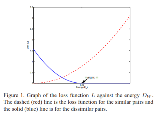
- Red: similar pairs
- Blue: dissimilar pairs
- Loss

- $L_S$: Partial loss of similar samples
- $L_D$: Partial loss of dissimilar samples
- $L_D = 0,$ $if D_W > m$
- Margin $m$: radius around $G_W(X)$
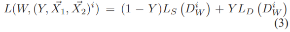
Spring Analogy
Equation of a spring
$F = -KX$
- F: force
- K: spring constant
- X: displacement (변위) of the spring from its rest length

- Similar points (attract-only spring)
- rest length = 0
- X > 0 → attractive force btw its ends
- $L_S$ gives attractive force
- Dissimilar points (m-repulse-only spring)
- rest length = m
- X < m → push apart
- X > m → no attractive force
- $L_D$ gives perturbation X of the spring from its rest length
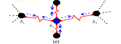
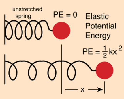
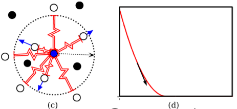
- Equilibrium
- Minimizing global loss function L
- A point is pulled by other points in different directions
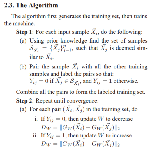
Algorithm
[Step 1] Prior knowledge: pair the similar samples (Y=0) and the dissimilar samples (Y=1)
[Step 2] Decrease distance $D_W$ between similar pairs and increase distance between dissimilar pairs by minimizing global loss function $L$
Analysis
[Figure 4] Mapping digit images to a 2D manifold
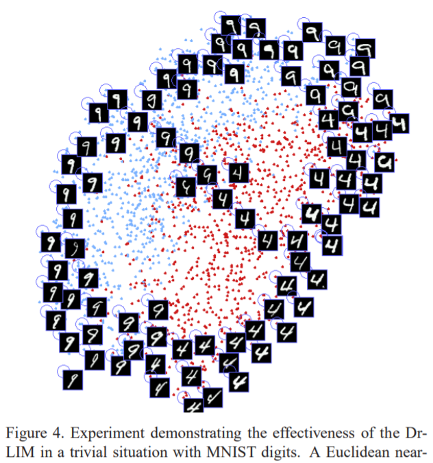
- Test samples - neighborhood relationships are unknown
- Euclidean distance is used to create local neighborhood relationships
- Evenly distributed on 2D manifold
- 9's and 4's regions are overlapped — slant angle (경사각) determines organization
[Figure 7] Mapping shifted digit images to a 2D manifold
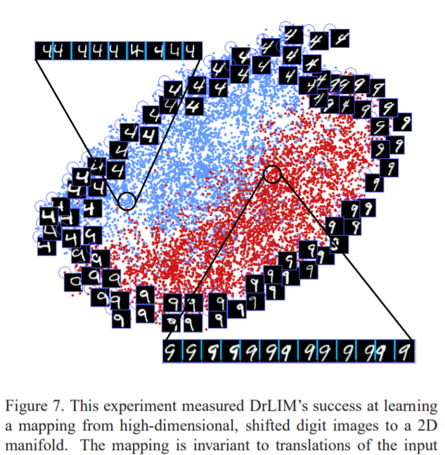
- Mapping is invariant to translations (the sequences of images)
- Globally coherent
[Figure 8] Mapping images of a single airplane to a 3D manifold
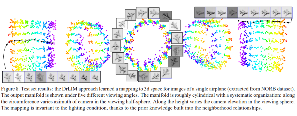
- Height of cylinder: elevation of input space
- Mapping is invariant to lighting (a horizontal line of a cylinder)
Q&A
(At the beginning of Section 2, the properties of parametric function $G_W$)
How are "a mapping using function is not constrained by implementing simple distance measures" and "learning invariances to complex transformations (of inputs)" connected?
- This method is not limited by euclidian distance of pairs, $X_i$ and $X_j$.
- Instead, it utilizes the convolutional nerual networks (CNNs) which is a non-linear transformation to capture neighborhood relationships and learn invariances to complex transformations.
- Complex transformations might be a non-linear transformation conducted by CNN and perturbations of the input image.
(Figure 1) the relationship between loss function $L$ and the energy $D_W$.
- $L = 1/2 * D_W^2$
- x-axis: $D_W$
- y-axis: $L_S, L_D$
- $L_S$ is increasing with $D_W$ (we want to decrease distance between similar points)
- $L_D$ is decreasing with $D_W$ if $D_W < m$, and is zero otherwise (we want to increase distance between dissimilar points)
(Page 3) In this sentence "Thus by minimizing the global loss function L over all springs, one would ultimately drive the system to its equilibrium state", the "equilibrium state" refers that similar samples are mapped closer, and dissimilar samples are mapped in distant?
- Equilibrium state is the state when input sample doesn't need to move and the similar samples around the input sample pull in different directions.
- From an optimization point of view, the partial derivative of the global loss function $L$ is zero, and the loss function converges to a local minimum.
'Papers > SSL' 카테고리의 다른 글
| [짧은 논문 리뷰] Motivation of ConVIRT (0) | 2022.01.13 |
|---|---|
| [코드 리뷰] SimCLR Code Review (3) | 2021.10.11 |
| [리뷰] In Defense of Pseudo-Labeling: An Uncertainty-Aware Pseudo-label Selection Framework for Semi-Supervised Learning (ICLR 2021) (0) | 2021.08.03 |


